JPEG Compression as a Differentiable PyTorch Module

Most autoencoders learn their representations from data. That’s powerful, but opaque — you can’t easily reason about what each latent dimension means, or guarantee invertibility.

JPEG takes the opposite approach. Its encoding is a fixed, well-understood signal-processing pipeline. I’ve always found that contrast interesting, so I built dct-autoencoder — a PyTorch module that implements the core JPEG pipeline analytically, without any training.

The motivation

A question I kept running into doing computer vision work: why do we process images in RGB?

For tasks like classification, segmentation, or detection, spatial resolution matters a lot. Show a human a 64×64 image and ask them to classify it — it’s genuinely hard. Show them a 512×512 image with heavy JPEG compression artifacts and they get it immediately. The structure is there, the fine color detail is not, and that’s fine.

RGB doesn’t reflect this. A 512×512×3 tensor treats every pixel’s red, green, and blue values as equally important. But a lot of that color information — especially in high frequencies — is not what the model needs.

My bet with this package: we can process high-resolution images with much lower compute by working in the frequency domain instead.

A 512×512 RGB image encoded with block size 8, keeping 24 luminance and 4 chrominance channels per block, becomes a 64×64×32 tensor. That’s the same scene, but 6× fewer values to process. The spatial structure is preserved. The perceptually irrelevant high-frequency color detail is dropped. And 32 channels is well within the range of standard CNN input stages — many architectures stack extra channels on top of RGB anyway.

This is the same trade-off JPEG has exploited for decades. The difference is that here it’s a differentiable PyTorch module, so gradients flow through it.

The pipeline

The full encode → compress → decompress → decode flow mirrors JPEG’s core structure:

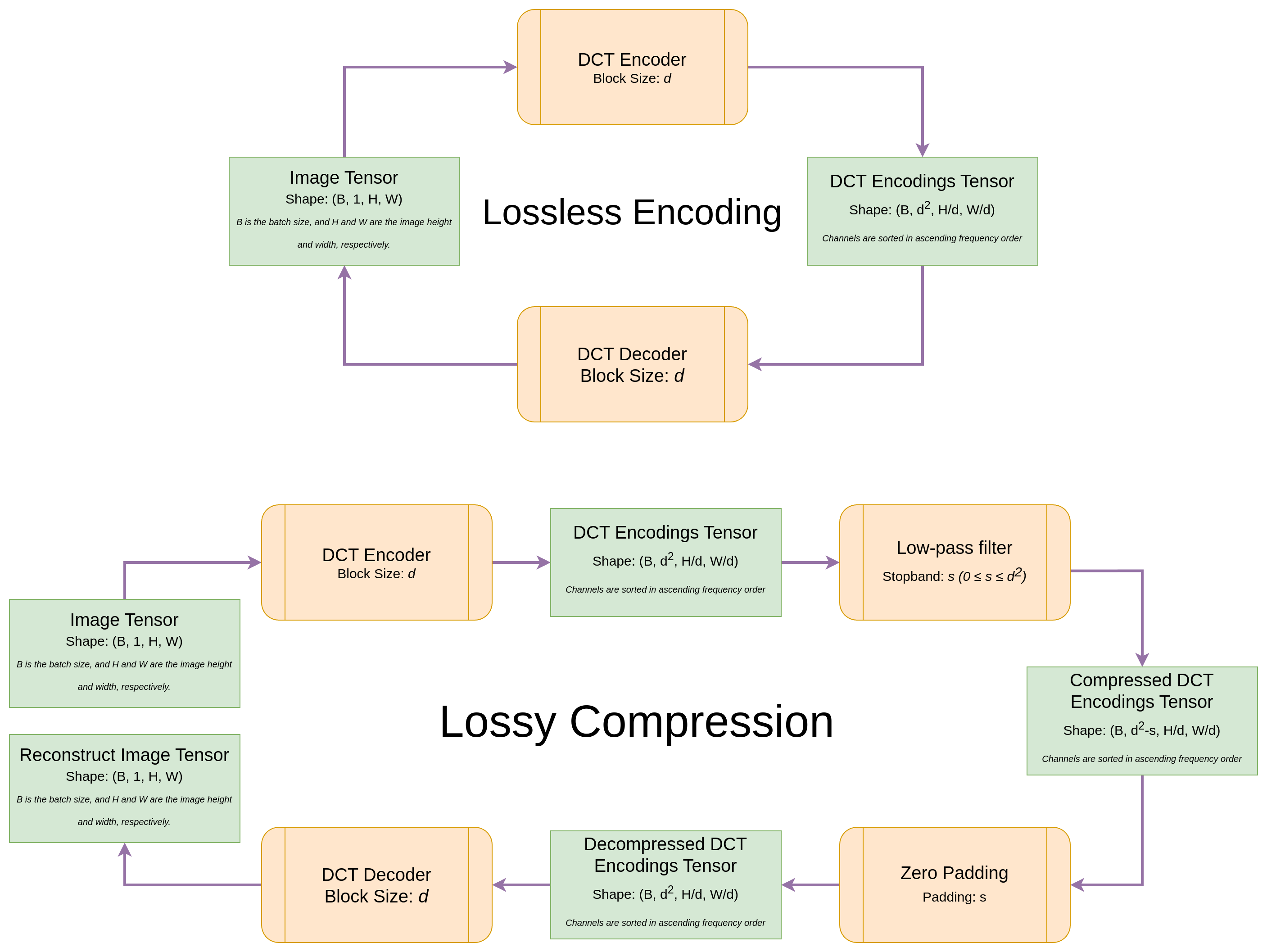
1. RGB → YCbCr — separate luminance (brightness) from chrominance (colour)
2. Block DCT — split each channel into non-overlapping $N \times N$ blocks and apply the 2-D Type-II DCT via strided convolution
3. Optional compression — zero out high-frequency coefficients
4. Inverse path — pad zeros back in, apply IDCT, convert YCbCr → RGB

Encoding is lossless by default. Compression is opt-in.

The math

Why YCbCr?

RGB channels are highly correlated. The human visual system is far more sensitive to brightness than to hue, so JPEG first separates the two:

• Y — luminance (perceived brightness)
• Cb — blue-difference chrominance
• Cr — red-difference chrominance

The forward transform:

The 0.5 offset keeps values in $[0, 1]$ when the input is in $[0, 1]$. The inverse uses the exact matrix inverse, so the round-trip is numerically exact within floating-point precision.

The 2-D DCT

For an $N \times N$ block, the Type-II 2-D DCT maps pixel values $f(x, y)$ to coefficients $F(u, v)$:

where $C(0) = 1/\sqrt{2}$ and $C(k) = 1$ for $k > 0$.

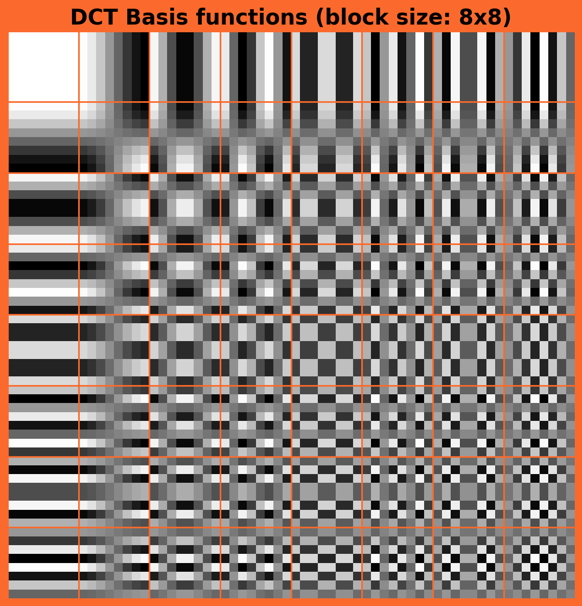
For the standard JPEG block size $N = 8$, there are 64 basis functions — one per frequency pair $(u, v)$. Each is the outer product of two 1-D cosine waves:

• $(u, v) = (0, 0)$ is the DC component — a flat patch capturing the block’s average intensity
• Higher $(u, v)$ oscillate faster, capturing finer spatial detail

All 64 basis functions for an $8 \times 8$ block:

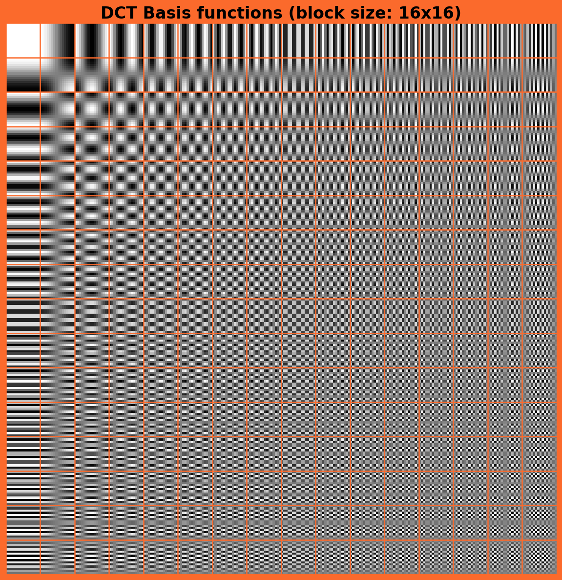
And for $N = 16$:

Why convolution?

Rather than looping over blocks in Python, the DCT is implemented as a strided convolution with precomputed cosine kernels. The full coefficient is:

where the inner product comes from F.conv2d and decoding uses F.conv_transpose2d — the exact inverse. This keeps the whole thing differentiable and GPU-friendly.

Channel ordering

The spatial frequency magnitude of each $(u, v)$ pair is $\|\mathbf{f}_{u,v}\| = \sqrt{u^2 + v^2}$. The autoencoder sorts kernels by this magnitude, so channel 0 is always DC and the last channels hold the finest detail:

channel 0  →  (u=0, v=0)  →  DC (flat)        ‖f‖ = 0
channel 1  →  (u=1, v=0)  →  slow horizontal  ‖f‖ = 1
channel 2  →  (u=0, v=1)  →  slow vertical    ‖f‖ = 1
...
channel 63 →  (u=7, v=7)  →  finest detail    ‖f‖ ≈ 9.9

This ordering means truncation is equivalent to low-pass filtering — you just keep the first $k$ channels.

Compression ratio

For block size $N$, retaining $k_Y$ luminance and $k_C$ chrominance channels, the compression ratio relative to the full encoding is:

Example ($k_Y = 10$, $k_C = 6$, $N = 8$):

Does it work?

Lossless round-trip

With default settings (no compression), encode → decode recovers the original within floating-point tolerance:

Max reconstruction error: 0.000001

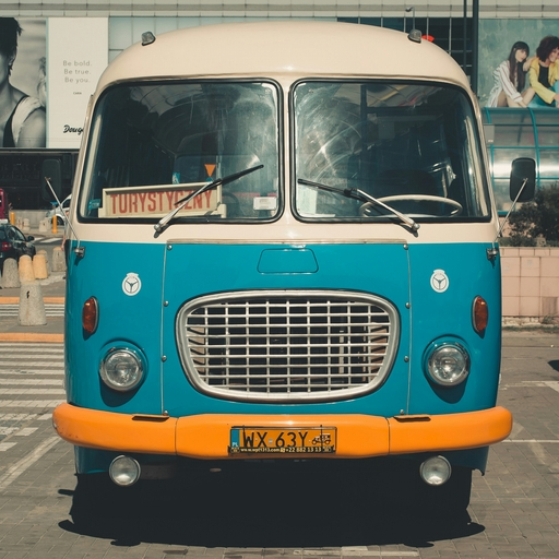
A max absolute error of ~$10^{-6}$ confirms the round-trip is invertible to floating-point precision.

Lossy compression

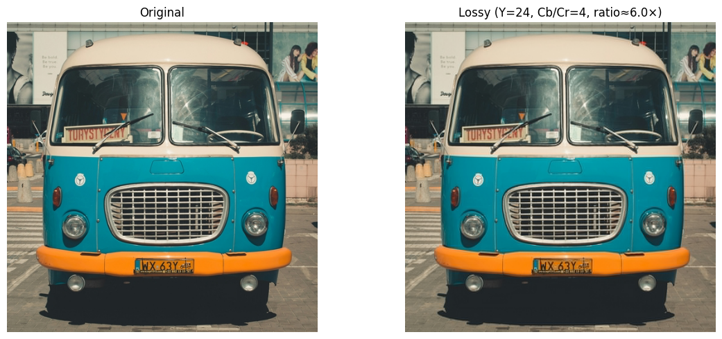
Retaining 24 luminance and 4 chrominance coefficients (of 64 each) gives a 6× compression ratio. The reconstruction retains overall structure and brightness while softening fine texture — exactly the trade-off JPEG is designed for:

A speculative application: super-resolution in frequency space

One idea I haven’t validated yet but find interesting: upsampling in the frequency domain rather than pixel space.

Standard super-resolution methods (SRCNN, ESRGAN, etc.) learn to hallucinate pixels. The network takes a low-resolution image and predicts what the missing high-frequency pixel detail probably looks like. It works, but it’s operating in a space where “what’s missing” is implicit.

What if instead you were explicit about it? Consider this pipeline:

512×512×3   →  encode(block=8)   →  64×64×192
            →  learnable 192→768  →  64×64×768
            →  decode(block=16)   →  1024×1024×3

You start with a 512×512 image, encode it into 64×64×192 DCT coefficients. A learnable network then expands those 192 channels to 768. You then decode using a block-16 DCT decoder, which interprets each 64×64 spatial position as a 16×16 block — giving you a 1024×1024 output. That’s a 2× spatial upscaling.

The interesting part: the network isn’t learning to hallucinate pixels. It’s learning to hallucinate DCT coefficients — and you know exactly what each coefficient means. A high-frequency coefficient at position $(u, v)$ corresponds to a specific spatial oscillation pattern. The network’s job is to decide which of those patterns are plausibly present given the low-frequency information it has.

Add compression to the mix and it gets more interesting still. You don’t need all 768 channels — the network can learn to populate only the coefficients it has enough information to recover confidently, and leave the rest zeroed.

Whether this works better than pixel-space super-resolution in practice is an open question. But the formulation feels cleaner to me — you’re explicit about what’s known, what’s missing, and what you’re asking the network to infer.

Quick start

pip install dct-autoencoder

import torch
from dct_autoencoder import DCTAutoencoder

model = DCTAutoencoder(
    block_size=8,
    num_luminance_compressed_channels=24,
    num_chrominance_compressed_channels=4,
)

images = torch.rand(1, 3, 256, 256)  # values in [0, 1]

encoded       = model.encode(images)
compressed    = model.compress(encoded)
reconstructed = model.decode(model.decompress(compressed))

The full tutorial notebook is here.

When is this useful?

Honestly, not everywhere. This is not a replacement for production JPEG encoders — it outputs tensors, not compressed file formats. And it won’t beat learned compression methods that optimize rate–distortion on real data.

But it’s useful when you need a fixed, interpretable frequency-domain representation inside a PyTorch pipeline, when gradients need to flow through a compression step, or simply when you want to understand how JPEG thinks about images without leaving Python.